Enzymatic#

For slightly more complex example, SimBio contains compound reactions, consisting of many single or compound reactions. For instance, from simbio.reactions.enzymatic we can import a MichaelisMenten reaction, which binds a substrate \(S\) to an enzyme \(E\) creating an intermediate bound species \(E:S\), before converting to the product \(P\) species:

\[ S + E ↔ E:S → P + E \]

It consists of a ReversibleSynthesis (\( S + E ↔ E:S\)) and a Dissociation (\(E:S → P + E\)) reaction. In turn, ReversibleSynthesis is also a compound reaction, consisting of a Synthesis (\( S + E → E:S\)) and Dissociation (\( E:S → S + E\)) reactions.

import numpy as np

from simbio.components import EmptyCompartment, Species
from simbio.reactions.enzymatic import MichaelisMenten
from simbio.simulator import Simulator

When defining a model, we do not need to explicitly create every species. For instance, the intermediate species ES, is created inside the reaction by assigning it to a number.

class Model(EmptyCompartment):
    enzyme: Species = 1
    subtrate: Species = 1
    product: Species = 0

    catalyze = MichaelisMenten(
        E=enzyme,
        S=subtrate,
        ES=0,  # "nameless" intermediate species
        P=product,
        forward_rate=1,
        reverse_rate=1,
        catalytic_rate=1,
    )

To simulate it, we feed the model into Simulator, and use the .run() method. It will compile and integrate an ODE-based simulation, returning a pandas.DataFrame with the result:

simulator = Simulator(Model)

t = np.linspace(0, 10, 100)
df = simulator.run(t)
df.head()

	enzyme	subtrate	catalyze.ES	product
time
0.00000	1.000000	1.000000	0.000000	0.000000
0.10101	0.916804	0.912323	0.083196	0.004481
0.20202	0.860984	0.845092	0.139016	0.015891
0.30303	0.823633	0.791686	0.176367	0.031947
0.40404	0.798962	0.747866	0.201038	0.051096

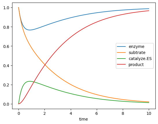
To visualize the time evolution, we can use the DataFrame.plot method:

df.plot()

<AxesSubplot: xlabel='time'>

SimBio documentation

Enzymatic

Enzymatic#